Deep learning has revolutionized image and speech processing, allowing you to turn edges into cats. In our lab, we’re applying these techniques to small molecule drug discovery.
A by-product of the revolution in deep learning has been the development of several high-quality open-source machine-learning frameworks that can compute gradients of arbitrary operations. Google’s Tensorflow may be the best known. My research has focused on understanding the results of large molecular dynamics simulations of proteins and other biomolecules. You can easily imagine framing the prediction of small molecule binding energies as a learning problem; can we leverage some of the deep learning advances for molecular dynamics for things in addition to artsy protein images?
A common operation in biophysics is computing the similarity of two protein poses (conformations) with the RMSD distance metric. This metric is beloved for its respect of translational and rotational invariances. Roughly, it overlays two protein structures and reports the mean distance between an atom and its partner in the other structure.
RMSD and rotations
Satisfying translational symmetry is easy: you just center your proteins at the origin prior to doing a comparison
# traj = np.array(...) [shape (n_frames, n_atoms, 3)]
traj -= np.mean(traj, axis=1, keepdims=True)
Satisfying rotational symmetry is harder. You need to find the optimal rotation between each pair of conformations (optimal = minimizes the RMSD). Back in 1976, Kabsch figured out that you could do an SVD of the 3x3 (xyz) correlation matrix to find the optimal rotation matrix.
# x1 = np.array(...) [shape (n_atoms, 3)]
correlation_matrix = np.dot(x1.T, x2)
V, S, W_tr = np.linalg.svd(correlation_matrix)
rotation = np.dot(V, W_tr)
x1_rot = np.dot(x1, rotation)
This isn’t ideal because the SVD might give you a “rotoinversion”, aka impropper rotation, aka rotation followed by an inversion. We have to explicitly check for and fix this case:
correlation_matrix = np.dot(x1.T, x2)
V, S, W_tr = np.linalg.svd(correlation_matrix)
is_reflection = (np.linalg.det(V) * np.linalg.det(W_tr)) < 0.0
if is_reflection:
    V[:, -1] = -V[:, -1]
rotation = np.dot(V, W_tr)
x1_rot = np.dot(x1, rotation)
Quaternions to the rescue
In 1987, Horn figured out that you can construct a 4x4 “key” matrix from combinations of elements of the correlation matrix. He derived this matrix from quaternion math (although the key matrix is a normal matrix). The leading eigenvalue of this matrix can be used to “rotationally correct” the naive squared difference between atomic coordinates.
correlation_matrix = np.dot(x1.T, x2)
F = key_matrix(correlation_matrix)
vals, vecs = np.linalg.eigh(F)
max_val = vals[-1] # numpy sorts ascending
sd = np.sum(traj1 ** 2 + traj2 ** 2) - 2 * max_val
msd = sd / n_atoms
rmsd = np.sqrt(msd)
Crucially, you don’t need to explicitly construct a rotation matrix to find the RMSD value. If you want the rotation, you can reconstruct it from the leading eigenvector of the key matrix.
Tensorflow can do this
We’ve formulated the problem as vector operations and one self-adjoint eigenvalue problem. All of these operations are implemented in Tensorflow!
def key_matrix(r):
    # @formatter:off
    return [
        [r[0][0] + r[1][1] + r[2][2], r[1][2] - r[2][1], r[2][0] - r[0][2], r[0][1] - r[1][0]],
        [r[1][2] - r[2][1], r[0][0] - r[1][1] - r[2][2], r[0][1] + r[1][0], r[0][2] + r[2][0]],
        [r[2][0] - r[0][2], r[0][1] + r[1][0], -r[0][0] + r[1][1] - r[2][2], r[1][2] + r[2][1]],
        [r[0][1] - r[1][0], r[0][2] + r[2][0], r[1][2] + r[2][1], -r[0][0] - r[1][1] + r[2][2]],
    ]


def squared_deviation(frame, target):
    R = tf.matmul(frame, target, transpose_a=True)
    R_parts = [tf.unstack(t) for t in tf.unstack(R)]
    F_parts = key_matrix(R_parts)
    F = tf.stack(F_parts, name='F')
    vals, vecs = tf.self_adjoint_eig(F, name='eig')
    lmax = tf.unstack(vals)[-1] # tensorflow sorts ascending
    sd = tf.reduce_sum(frame ** 2 + target ** 2) - 2 * lmax
The benefit is now we get derivatives for free, so we can do interesting things. As a toy example, this shows finding a “consensus” structure that minimizes average RMSD to every frame in a molecular dynamics trajectory
This is the normal, tensorflow code used to perform the optimization.
target = tf.Variable(tf.truncated_normal((1, n_atoms, 3), stddev=0.3), name='target')
msd, rot = pairwise_msd(traj, target)
loss = tf.reduce_mean(msd, axis=0)

optimizer = tf.train.AdamOptimizer(1e-3)
train = optimizer.minimize(loss)

sess = tf.Session()
sess.run(tf.global_variables_initializer())
for step in range(2500):
    sess.run(train)
Tensorflow can’t actually do this very well
Doing an eigendecomposition for each data point gets expensive, especially since I want to be able to do pairwise (R)MSD calculations between a large trajectory and a sizeable number of target structures. MDTraj can perform a huge number of RMSD calculations exceedingly quickly. It uses a better strategy for finding the leading eigenvalue of the 4x4 key matrix from above. The Theobald QCP method from 2005 explicitly writes out the characteristic polynomial for the key matrix. We use the fact that there is a bound for identical structures ((R)MSD = 0) to choose a starting point for an iterative, Newton method of finding the leading eigenvalue. If we start from this point, we’re guarenteed that the first root of the characteristic polynomial will be the largest eigenvalue. So let’s code this up in Tensorflow! Not so fast (literally): you can’t really do iteration in Tensorflow, and who knows how performant it would be if you could.
Custom Pairwise MSD Op
Instead, I implemented a custom Tensorflow “op”. At first, I was intimidated by having to build and keep track of a custom Tensorflow installation. Luckily, Tensorflow will happily load shared libraries to register Ops at runtime. Even better, a Pande Group Alumn Imran Haque implemented a fast (R)MSD calculation implementation in C that I could wrap.
I implemented an Op that does pairwise MSD calculations where the double-for-loop is parallelized with OpenMP. In addition to the 10,000x speedup from the native tensorflow implementation of the Horn method, we’re slightly faster than MDTraj even though it’s using the same implementation under the hood. For MDTraj, the looping over a trajectory is done with OpenMP in C, but the iteration over targets has to be done in Python with its associated overhead.
I ran a benchmark which performs a pairwise RMSD calculation among fs peptide trajectories. Specifically, between 2800 (stride = 100) frames and 28 targets (stride = 100 * 100).
| Implementation | Time / ms |
|---|---|
| TF Native Ops | 22,843 |
| MDTraj | 33.3 |
| TF Custom Op | 0.9 |
| TF Custom Op (w/rot) | 1.6 |
What about gradients?
The reason why we wanted to use Tensorflow in the first place was to do fun things with the automatic differentiation. There’s no free lunch, and Tensorflow will not auto-differentiate our custom Op. Coutsias et. al. pointed out that the derivative of the MSD is simply the difference between the coordinates in the superposed pair of structures. We can code this.
The first problem is now we need the rotation matrix explicitly so we can use it to compute the gradients. Remember that Theobald came up with a smart method for finding the leading eigenvalue, but that only gives us the RMSD value, not the actual rotation (which requires the eigenvector). Luckily, in 2010 he extended the method to use the leading eigenvalue to quickly find the leading eigenvector.
I modified the pairwise_msd op to return a (n_frames, n_targets) pairwise MSD matrix and the (n_frames, n_targets, 3, 3) rotation matrices. Users should never use the rotation matrices for further calculations because I didn’t implement the derivatives for that output. Instead, I use that output in the gradient calculation for the MSDs. If someone knows a better way to do this, please let me know.
In the benchmark table, this version of the Op is the “w/rot” variant, and is slower (because it has to do more work).
Way too much detail about the gradient code
Most of this code is just making tensors the right shape. We need to apply our n_frames * n_targets rotation matrices individually to each conformation, and we need to mix in the gradient grad from the previous Op in the compute graph, so we blow everything up to a rank 4 matrix and explicitly tile the conformations to be rotated because matmul doesn’t do broadcasting.
rots = op.outputs[1]
N1 = int(confs1.get_shape()[0])
N2 = int(confs2.get_shape()[0])

# expand from (n_frames, n_targets) to (n_frame, n_targets, 1, 1)
grad = tf.expand_dims(tf.expand_dims(grad, axis=-1), axis=-1)

# expand from (n_frames OR n_targets, n_atoms, 3)
# to (n_frames OR 1, 1 OR n_targets, n_atoms, 3)
expand_confs1 = tf.expand_dims(confs1, axis=1)
expand_confs2 = tf.expand_dims(confs2, axis=0)

# Explicitly tile conformations for matmul
big_confs1 = tf.tile(expand_confs1, [1, N2, 1, 1])
big_confs2 = tf.tile(expand_confs2, [N1, 1, 1, 1])

# This is the gradient!
dxy = expand_confs1 - tf.matmul(big_confs2, rots, transpose_b=True)
dyx = expand_confs2 - tf.matmul(big_confs1, rots, transpose_b=False)
The actual form of the gradient has a couple factors which we must include:
n_atom = float(int(confs1.get_shape()[1]))
dxy = 2 * dxy / n_atom
dyx = 2 * dyx / n_atom
Finally, we sum over the axis that has the other conformations to make sure our gradient tensors match in shape to their variables.
dr_dc1 = tf.reduce_sum(grad * dxy, axis=1)
dr_dc2 = tf.reduce_sum(grad * dyx, axis=0)
Did you forget about translational symmetry after all this focus on rotation? I did originally! Test your code on a variety of inputs including trajectories that aren’t pre-centered :). Let’s use Tensorflow’s automatic differentiation for this part.
Specifically, we set up the “forward” op and call tf.gradients on it. We pass in our gradients w.r.t. rotation as the grad_ys argument. Yay chain rule!
centered1 = confs1 - tf.reduce_mean(confs1, axis=1, keep_dims=True)
centered2 = confs2 - tf.reduce_mean(confs2, axis=1, keep_dims=True)
dc_dx1 = tf.gradients(centered1, [confs1], grad_ys=dr_dc1)[0]
dc_dx2 = tf.gradients(centered2, [confs2], grad_ys=dr_dc2)[0]
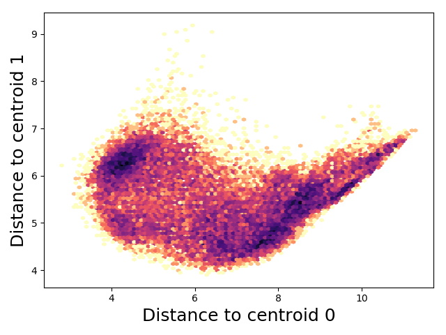
KMeans-inspired RMSD clustering
As an example of what we can do with our fast pairwise MSD op with gradients, let’s find “optimal” cluter centers (centroids). For a trajectory of conformations, find centers that minimize the distance between each point and its closest centroid. To prevent it from finding the same centroid twice, we add a penalty to force the centroids apart. Be careful to make sure this penalty saturates at some point or your optimization will just make really different centroids with no respect for inter-cluster distances.
# Out inputs
n_clusters = 2
target = tf.Variable(tf.truncated_normal((n_clusters, traj.xyz.shape[1], 3), stddev=0.3))

# Set up the compute graph
msd, rot = rmsd_op.pairwise_msd(traj.xyz, target)
nearest_cluster = msd * tf.nn.softmax(-msd)
cluster_dist = tf.reduce_mean(nearest_cluster, axis=(0, 1))
cluster_diff, _ = rmsd_op.pairwise_msd(target, target)
cluster_diff = cluster_diff[0, 1]
loss = cluster_dist - tf.tanh(cluster_diff*10)

# Train it in the normal way
optimizer = tf.train.AdamOptimizer(5e-3)
train = optimizer.minimize(loss)

sess = tf.Session()
sess.run(tf.global_variables_initializer())
for step in range(1000):
    sess.run(train)
Now you can do tICA or make an MSM in this nice space.
Code Availability
All code is available on Github. Make sure you check out the README for installation instructions, as the custom Op requires a working c++ compiler. The consensus example, clustering example, and profiling script are found in the examples folder and require the fs peptide dataset.
The native tensorflow implementation lives in rmsd.py. The low level code for the custom Op lives in the rmsd/ subfolder, specifically rmsd.cpp. Finally, rmsd_op.py contains a convenience function for loading the shared object that registers the Op. It also implements the gradients (in Python).