Question
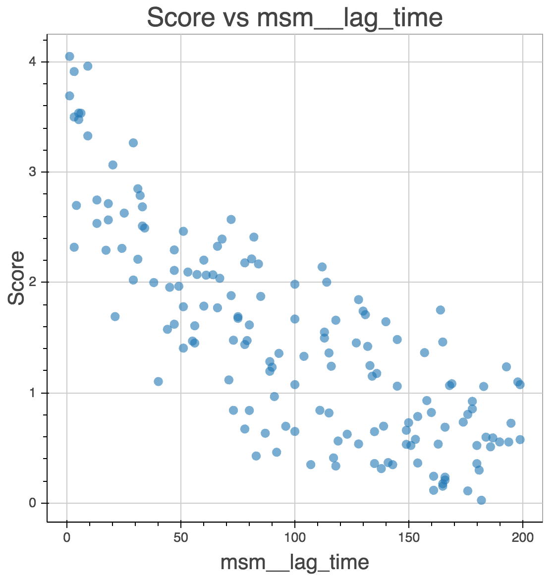
Github user jeiros asked why you can’t use GMRQ to find the best lag-time when building an MSM. He wanted to know why the score appears to decrease with increasing lag-time:

The full question is here.
Answer
Eigenvalues behave predictably with lag-time. Assume you have a transition matrix $\mathbf{T}$ parameterized at lag time $\tau$. Operating on a vector $\mathbf{x}$ twice should give you the same result as using a transition matrix parameterized at lag-time $2\tau$. This is a consequence of Markovianity.
\[\mathbf{T}(\tau)\mathbf{T}(\tau)\mathbf{x} = \mathbf{T}(2\tau)\mathbf{x}\]So
\[\mathbf{T}^2(\tau) = \mathbf{T}(2\tau)\]And the eigenvalues
\[\lambda^2(\tau) = \lambda(2\tau)\]This is why we define the timescales $t_i$ such that
\[\lambda_i(\tau) = e^{-\tau/t_i} \\ t_i = \frac{-\tau}{\ln{\lambda_i(\tau)}}\]If $\mathbf{T}^2=\mathbf{T}(2\tau)$, then the timescales should be invariant to lag-time.
The GMRQ score is the sum of the first $m$ eigenvalues
\[\sum_{i=1}^{m}{\lambda_i} = \sum{e^{-\tau/t_i}}\]As $\tau$ gets larger, the exponent gets more negative, and the GMRQ score decreases.
In practice, the timescales do vary with the lag-time parameter, but not in any way we can account for. You can’t optimize the lag-time parameter because it is not a parameter. The object that we are scoring is $\mathbf{T}(\tau)$. If you change $\tau$, you’re scoring a different entity.
For full details, you can read the GMRQ paper doi:10.1063/1.4916292. Also check out the continuous time version of MSMs which uses lag-time as a tunable parameter and its associated paper doi:10.1063/1.4926516.